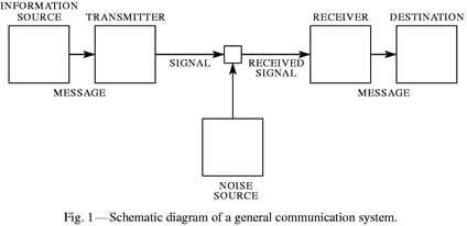
A Mathematical Theory of Communication

C. E. SHANNON 1948

Reprinted with corrections from The Bell System Technical Journal, Vol. 27, pp. 379-423, 623-656, July, October, 1948.

Note from the editor:

This page is part of a collection of articles on the Thocp site because of its historic importance.

This article wase selected because it made binairy (electronic) computing possible

TD align="left" valign="top" width="14%">

INTRODUCTION

TD colspan="10" align="left" valign="top" width="92%"> THE recent development of various methods of modulation such as PCM and PPM which exchange bandwidth for signal-to-noise ratio has intensified the interest in a general theory of communication. A basis for such a theory is contained in the important papers of Nyquist ¹ and Hartley ² on this subject. In the present paper we will extend the theory to include a number of new factors, in particular the effect of noise in the channel, and the savings possible due to the statistical structure of the original message and due to the nature of the final destination of the information. TD colspan="10" align="left" valign="top" width="92%"> The fundamental problem of communication is that of reproducing at one point either exactly or ap proximately a message selected at another point. Frequently the messages have meaning; that is they refer to or are correlated according to some system with certain physical or conceptual entities. These semantic aspects of communication are irrelevant to the engineering problem. The significant aspect is that the actual message is one selected from a set of possible messages. The system must be designed to operate for each possible selection, not just the one which will actually be chosen since this is unknown at the time of design. TD colspan="10" align="left" valign="top" width="92%"> If the number of messages in the set is finite then this number or any monotonic function of this number can be regarded as a measure of the information produced when one message is chosen from the set, all choices being equally likely. As was pointed out by Hartley the most natural choice is the logarithmic function. Although this definition must be generalized considerably when we consider the influence of the statistics of the message and when we have a continuous range of messages, we will in all cases use an essentially logarithmic measure. TD colspan="06" align="left" valign="top" width="56%"> The logarithmic measure is more convenient for various reasons: TD colspan="09" align="left" valign="top" width="89%"> 1. It is practically more useful. Parameters of engineering importance such as time, bandwidth, number of relays, etc., tend to vary linearly with the logarithm of the number of possibilities. For example, adding one relay to a group doubles the number of possible states of the relays. It adds 1 to the base 2 logarithm of this number. Doubling the time roughly squares the number of possible messages, or doubles the logarithm, etc. TD colspan="09" align="left" valign="top" width="89%"> 2. It is nearer to our intuitive feeling as to the proper measure. This is closely related to (1) since we in tuitively measures entities by linear comparison with common standards. One feels, for example, that two punched cards should have twice the capacity of one for information storage, and two identical channels twice the capacity of one for transmitting information. TD colspan="09" align="left" valign="top" width="89%"> 3. It is mathematically more suitable. Many of the limiting operations are simple in terms of the loga rithm but would require clumsy restatement in terms of the number of possibilities. TD colspan="10" align="left" valign="top" width="92%"> The choice of a logarithmic base corresponds to the choice of a unit for measuring information. If the base 2 is used the resulting units may be called binary digits, or more briefly bits, a word suggested by J. W. Tukey. A device with two stable positions, such as a relay or a flip-flop circuit, can store one bit of information. N such devices can store N bits, since the total number of possible states is 2 ^N and 109 ₂ 2 ^N= N. If the base 10 is used the units may be called decimal digits. Since TD colspan="03" align="left" valign="top" width="22%">

log ₂ M =log ₁₀ M/ log ₁₀ ² = 3.32log ₁₀ M, ⁽²⁾



a decimal digit is about 33 bits. A digit wheel on a desk computing machine has ten stable positions and therefore has a storage capacity of one decimal digit. In analytical work where integration and differentiation are involved the base e is sometimes useful. The resulting units of information will be called natural units. Change from the base a to base b merely requires multiplication by log _o a.
By a communication system we will mean a system of the type indicated schematically in Fig. 1. It consists of essentially five parts:

1. An information source which produces a message or sequence of messages to be communicated to the receiving terminal. The message may be of various types: (a) A sequence of letters as in a telegraph of teletype system; (b) A single function of time f (t) as in radio or telephony; (c) A function of time and other variables as in black and white television - here the message may be thought of as a function f (x,y, t) of two space coordinates and time, the light intensity at point (x,y) and time t on a pickup tube plate; (d) Two or more functions of time, say f (t), g(t), h(t) - this is the case in "three dimensional" sound transmission or if the system is intended to service several individual channels in multiplex; (e) Several functions of several variables-in color television the message consists of three functions f (x,y,t), g(x,y,t), h(x,y,t) defined in a three-dimensional continuum- we may also think of these three functions as components of a vector field defined in the region - similarly, several black and white television sources would produce "messages" consisting of a number of functions of three variables; (f) Various combinations also occur, for example in television with an associated audio channel.

2. A transmitter which operates on the message in some way to produce a signal suitable for trans mission over the channel. In telephony this operation consists merely of changing sound pressure into a proportional electrical current. In telegraphy we have an encoding operation which produces a sequence of dots, dashes and spaces on the channel corresponding to the message. In a multiplex PCM system the different speech functions must be sampled, compressed, quantized and encoded, and finally interleaved properly to construct the signal. Vocoder systems, television and frequency modulation are other examples of complex operations applied to the message to obtain the signal.

3. The channel is merely the medium used to transmit the signal from transmitter to receiver. It may be a pair of wires, a coaxial cable, a band of radio frequencies, a beam of light, etc.

4. The receiver ordinarily performs the inverse operation of that done by the transmitter, reconstructing the message from the signal.

5. The destination is the person (or thing) for whom the message is intended.

/TR> /TR>

We wish to consider certain general problems involving communication systems. To do this it is first necessary to represent the various elements involved as mathematical entities, suitably idealized from their physical counterparts. We may roughly classify communication systems into three main categories: discrete, continuous and mixed. By a discrete system we will mean one in which both the message and the signal are a sequence of discrete symbols. A typical case is telegraphy where the message is a sequence of letters and the signal a sequence of dots, dashes and spaces. A continuous system is one in which the message and signal are both treated as continuous functions, e.g., radio or television. A mixed system is one in which both discrete and continuous variables appear, e.g., PCM transmission of speech.
We first consider the discrete case. This case has applications not only in communication theory, but also in the theory of computing machines, the design of telephone exchanges and other fields. In addition the discrete case forms a foundation for the continuous and mixed cases which will be treated in the second half of the paper.
PART I: DISCRETE NOISELESS SYSTEMS 1. THE DISCRETE NOISELESS CHANNEL Teletype and telegraphy are two simple examples of a discrete channel for transmitting information. Gen erally, a discrete channel will mean a system whereby a sequence of choices from a finite set of elementary symbols S1, . . , S„ can be transmitted from one point to another. Each of the symbols Si is assumed to have a certain duration in time ti seconds (not necessarily the same for different Si, for example the dots and dashes in telegraphy). It is not required that all possible sequences of the Si be capable of transmission on the system; certain sequences only may be allowed. These will be possible signals for the channel. Thus in telegraphy suppose the symbols are: (1) A dot, consisting of line closure for a unit of time and then line open for a unit of time; (2) A dash, consisting of three time units of closure and one unit open; (3) A letter space consisting of, say, three units of line open; (4) A word space of six units of line open. We might place the restriction on allowable sequences that no spaces follow each other (for if two letter spaces are adjacent, it is identical with a word space). The question we now consider is how one can measure the capacity of such a channel to transmit information.

In the teletype case where all symbols are of the same duration, and any sequence of the 32 symbols is allowed the answer is easy. Each symbol represents five bits of information. If the system transmits n symbols per second it is natural to say that the channel has a capacity of 5n bits per second. This does not mean that the teletype channel will always be transmitting information at this rate - this is the maximum possible rate and whether or not the actual rate reaches this maximum depends on the source of information which feeds the channel, as will appear later.
In the more general case with different lengths of symbols and constraints on the allowed sequences, we make the following definition:
Definition: The capacity C of a discrete channel is given by


where N(T) is the number of allowed signals of duration T.
It is easily seen that in the teletype case this reduces to the previous result. It can be shown that the limit in question will exist as a finite number in most cases of interest. Suppose all sequences of the symbols Sl,. . . , S„ are allowed and these symbols have durations What is the channel capacity? If N(t) represents the number of sequences of duration t we have



The total number is equal to the sum of the numbers of sequences ending in Si, S2, . . . , S„ and these are N(t-ti),N(t-t2),...,N(t-tn), respectively. According to a well-known result in finite differences, N(t) is then asymptotic for large t to Xt/o where Xt/o is the largest real solution of the characteristic equation:

and therefore C = logX0.

In case there are restrictions on allowed sequences we may still often obtain a difference equation of this type and find C from the characteristic equation. In the telegraphy case mentioned above

N(t) = N(t- 2) +N(t-4) +N(t- 5) +N(t-7) +N(t- 8) +N(t- 10)

as we see by counting sequences of symbols according to the last or next to the last symbol occurring. Hence C is - log mu o where mu 0 is the positive root of 1= mu 2 + mu 4 + mu 5 + m ^{u 7} + mu ⁸ + m ^u 10 Solving this we find C = 0.539.

A very general type of restriction which may be placed on allowed sequences is the following: We imagine a number of possible states at, a2, . . ., am For each state only certain symbols from the set Sl, . . . , Sn can be transmitted (different subsets for the different states). When one of these has been transmitted the state changes to a new state depending both on the old state and the particular symbol transmitted. The telegraph case is a simple example of this. There are two states depending on whether or not a space was the last symbol transmitted. If so, then only a dot or a dash can be sent next and the state always changes. If not, any symbol can be transmitted and the state changes if a space is sent, otherwise it remains the same. The conditions can be indicated in a linear graph as shown in Fig. 2. The junction points correspond to the DASH WORD SPACE

Fig. 2-Graphical representation of the constraints on telegraph symbols.

states and the lines indicate the symbols possible in a state and the resulting state. In Appendix 1 it is shown that if the conditions on allowed sequences can be described in this form C will exist and can be calculated in accordance with the following result:

Theorem 1: Let b(i ^j)~(s)i be the duration of the s ^t ' symbol which is allowable in state i and leads to state j. Then the channel capacity C is equal to log W where W is the largest real root of the determinant equation:

Where =1 if i = j and is zero otherwise.

For example, in the telegraph case (Fig. 2) the determant is:

On expansion this leads to the equation given above for this case.

2. THE DISCRETE SOURCE OF INFORMATION

We have seen that under very general conditions the logarithm of the number of possible signals in a discrete channel increases linearly with time. The capacity to transmit information can be specified by giving this rate of increase, the number of bits per second required to specify the particular signal used.

We now consider the information source. How is an information source to be described mathematically, and how much information in bits per second is produced in a given source? The main point at issue is the effect of statistical knowledge about the source in reducing the required capacity of the channel, by the use of proper encoding of the information. In telegraphy, for example, the messages to be transmitted consist of sequences of letters. These sequences, however, are not completely random. In general, they form sentences and have the statistical structure of, say, English. The letter E occurs more frequently than Q, the sequence TH more frequently than XP, etc. The existence of this structure allows one to make a saving in time (or channel capacity) by properly encoding the message sequences into signal sequences. This is already done to a limited extent in telegraphy by using the shortest channel symbol, a dot, for the most common English letter E; while the infrequent letters, Q, X, Z are represented by longer sequences of dots and dashes. This idea is carried still further in certain commercial codes where common words and phrases are represented by four- or five-letter code groups with a considerable saving in average time. The standardized greeting and anniversary telegrams now in use extend this to the point of encoding a sentence or two into a relatively short sequence of numbers.
We can think of a discrete source as generating the message, symbol by symbol. It will choose succes sive symbols according to certain probabilities depending, in general, on preceding choices as well as the particular symbols in question. A physical system, or a mathematical model of a system which produces such a sequence of symbols governed by a set of probabilities, is known as a stochastic process. ³ We may consider a discrete source, therefore, to be represented by a stochastic process. Conversely, any stochastic process which produces a discrete sequence of symbols chosen from a finite set may be considered a discrete source. This will include such cases as:

1. Natural written languages such as English, German, Chinese.

2. Continuous information sources that have been rendered discrete by some quantizing process. For example, the quantized speech from a PCM transmitter, or a quantized television signal.

3. Mathematical cases where we merely define abstractly a stochastic process which generates a se quence of symbols. The following are examples of this last type of source.

(A) Suppose we have five letters A, B, C, D, E which are chosen each with probability .2, successive choices being independent. This would lead to a sequence of which the following is a typical example.

BDCBCECCCADCBDDAAECEEA ABBDAEECACEEBAEECBCEAD.

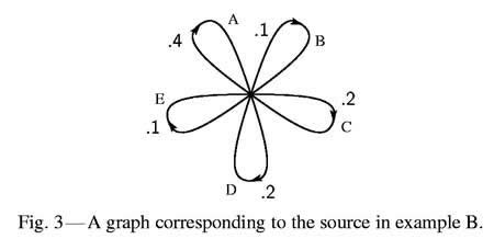
This was constructed with the use of a table of random numbers. (B) Using the same five letters let the probabilities be .4, .1, .2, .2, .1, respectively, with successive choices independent. A typical message from this source is then: AAACDCBDCEAADADACEDA EADCABEDADDCECAAAAAD.
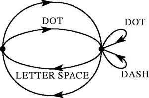
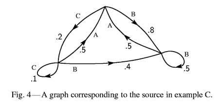
(C) A more complicated structure is obtained if successive symbols are not chosen independently but their probabilities depend on preceding letters. In the simplest case of this type a choice depends only on the preceding letter and not on ones before that. The statistical structure can then be described by a set of transition probabilities pi (j), the probability that letter i is followed by letter j. 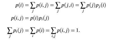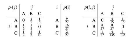The indices i and j range over all the possible symbols. A second equivalent way of specifying the structure is to give the "digram" probabilities p(i, j), i.e., the relative frequency of the digram i j. The letter frequencies p(i), (the probability of letter i), the transition probabilities

³ See, for example, S. Chandrasekhar, "Stochastic Problems in Physics and Astronomy," Reviews of Modern Physics, v. 15, No. 1, January 1943, p. 1.
⁴ Kendall and Smith, Tables of Random Sampling Numbers, Cambridge, 1939. 5

pi (j) and the digram probabilities p(i, j) are related by the following formulas:

As a specific example suppose there are three letters A, B, C with the probability tables:

A typical message from this source is the following: ABBABABABABABABBBABBBBBABABABABABBBACACAB BABBBBABBABACBBBABA.

The next increase in complexity would involve trigram frequencies but no more. The choice of a letter would depend on the preceding two letters but not on the message before that point. A set of trigram frequencies p(i, j, k) or equivalently a set of transition probabilities pii(k) would be required. Continuing in this way one obtains successively more complicated stochastic pro cesses. In the general n-gram case a set of n-gram probabilities p(il, i2, . . . , i _n ) or of transition probabilities Pi1,i2,.-i„_1 (in) is required to specify the statistical structure.

(D) Stochastic processes can also be defined which produce a text consisting of a sequence of "words." Suppose there are five letters A, B, C, D, E and 16 "words" in the language with associated probabilities:

JO A .16 BEBE .11 CABED .04 DEB

.04 ADEB .04 BED .05 GEED .15 DEED

.05 ADEE .02 BEED .08 DAB .01 EAB

.01 BADD .05 CA .04 DAD .05 EE

Suppose successive "words" are chosen independently and are separated by a space. A typical message might be:

DAB EE A BEBE DEED DEB ADEE ADEE EE DEB BEBE BEBE BEBE ADEE BED DEED DEED GEED ADEE A DEED DEED BEBE CABED BEBE BED DAB DEED ADEB.

If all the words are of finite length this process is equivalent to one of the preceding type, but the description may be simpler in terms of the word structure and probabilities. We may also generalize here and introduce transition probabilities between words, etc.

These artificial languages are useful in constructing simple problems and examples to illustrate vari ous possibilities. We can also approximate to a natural language by means of a series of simple artificial languages. The zero-order approximation is obtained by choosing all letters with the same probability and independently. The first-order approximation is obtained by choosing successive letters independently but each letter having the same probability that it has in the natural languages Thus, in the first-order ap proximation to English, E is chosen with probability .12 (its frequency in normal English) and W with probability .02, but there is no influence between adjacent letters and no tendency to form the preferred

⁵ Letter, digram and trigram frequencies are given in Secret and Urgent by Fletcher Pratt, Blue Ribbon Books, 1939. Word frequen cies are tabulated in Relative Frequency of English Speech Sounds, G. Dewey, Harvard University Press, 1923.

/TR> TD colspan="04" align="left" valign="top" width="50%"> 3. THE SERIES OF APPROXIMATIONS TO ENGLISH /TR> /TR> /TR> TD colspan="07" align="left" valign="top" width="89%"> XFOML RXKHRJFFJUJ ZLPWCFWKCYJ FFJEYVKCQSGHYD QPAAMKBZAACIBZL HJQD. /TR> /TR> TD colspan="07" align="left" valign="top" width="89%"> OCRO HLI RGWR NMIELWIS EU LL NBNESEBYA TH EEI ALHENHTTPA OOBTTVA NAH BRL. /TR> /TR> TD colspan="07" align="left" valign="top" width="89%"> ON IE ANTSOUTINYS ARE T INCTORE ST BE S DEAMY ACHIN D ILONASIVE TU COOWE AT TEASONARE FUSO TIZIN ANDY TOBE SEACE CTISBE. /TR> /TR> TD colspan="07" align="left" valign="top" width="89%"> IN NO IST LAT WHEY CRATICT FROURE BIRS GROCID PONDENOME OF DEMONS TURES OF THE REPTAGIN IS REGOACTIONA OF CRE. /TR> /TR> TD colspan="07" align="left" valign="top" width="89%"> REPRESENTING AND SPEEDILY IS AN GOOD APT OR COME CAN DIFFERENT NAT URAL HERE HE THE A IN CAME THE TO OF TO EXPERT GRAY COME TO FURNISHES THE LINE MESSAGE HAD BE THESE. /TR> /TR> TD colspan="07" align="left" valign="top" width="89%"> THE HEAD AND IN FRONTAL ATTACK ON AN ENGLISH WRITER THAT THE CHAR ACTER OF THIS POINT IS THEREFORE ANOTHER METHOD FOR THE LETTERS THAT THE TIME OF WHO EVER TOLD THE PROBLEM FOR AN UNEXPECTED. /TR>

digrams such as TH, ED, etc. In the second-order approximation, digram structure is introduced. After a letter is chosen, the next one is chosen in accordance with the frequencies with which the various letters follow the first one. This requires a table of digram frequencies pi (j). In the third-order approximation, trigram structure is introduced. Each letter is chosen with probabilities which depend on the preceding two letters.
To give a visual idea of how this series of processes approaches a language, typical sequences in the approx imations to English have been constructed and are given below. In all cases we have assumed a 27-symbol "alphabet," the 26 letters and a space.
1. Zero-order approximation (symbols independent and equiprobable).
2. First-order approximation (symbols independent but with frequencies of English text).
3. Second-order approximation (digram structure as in English).
4. Third-order approximation (trigram structure as in English).
5. First-order word approximation. Rather than continue with tetragram,. . . , n-gram structure it is easier and better to jump at this point to word units. Here words are chosen independently but with their appropriate frequencies.
6. Second-order word approximation. The word transition probabilities are correct but no further struc ture is included.
The resemblance to ordinary English text increases quite noticeably at each of the above steps. Note that these samples have reasonably good structure out to about twice the range that is taken into account in their construction. Thus in (3) the statistical process insures reasonable text for two-letter sequences, but four letter sequences from the sample can usually be fitted into good sentences. In (6) sequences of four or more words can easily be placed in sentences without unusual or strained constructions. The particular sequence of ten words "attack on an English writer that the character of this" is not at all unreasonable. It appears then that a sufficiently complex stochastic process will give a satisfactory representation of a discrete source.
The first two samples were constructed by the use of a book of random numbers in conjunction with (for example 2) a table of letter frequencies. This method might have been continued for (3), (4) and (5), since digram, trigram and word frequency tables are available, but a simpler equivalent method was used. 7

To construct (3) for example, one opens a book at random and selects a letter at random on the page. This letter is recorded. The book is then opened to another page and one reads until this letter is encountered. The succeeding letter is then recorded. Turning to another page this second letter is searched for and the succeeding letter recorded, etc. A similar process was used for (4), (5) and (6). It would be interesting if further approximations could be constructed, but the labor involved becomes enormous at the next stage.
4. GRAPHICAL REPRESENTATION OF A MARKOFF PROCESS
Stochastic processes of the type described above are known mathematically as discrete Markoff processes and have been extensively studied in the literature. ⁶ The general case can be described as follows: There exist a finite number of possible "states" of a system; St, S2,...,S„. In addition there is a set of transition probabilities; pi(j) the probability that if the system is in state Si it will next go to state Sp To make this Markoff process into an information source we need only assume that a letter is produced for each transition from one state to another. The states will correspond to the "residue of influence" from preceding letters.
The situation can be represented graphically as shown in Figs. 3, 4 and 5. The "states" are the junction

points in the graph and the probabilities and letters produced for a transition are given beside the correspond ing line. Figure 3 is for the example B in Section 2, while Fig. 4 corresponds to the example C. In Fig. 3

there is only one state since successive letters are independent. In Fig. 4 there are as many states as letters. If a trigram example were constructed there would be at most n ² states corresponding to the possible pairs of letters preceding the one being chosen. Figure 5 is a graph for the case of word structure in example D. Here S corresponds to the "space" symbol.
5. ERGODIC AND MIXED SOURCES
As we have indicated above a discrete source for our purposes can be considered to be represented by a Markoff process. Among the possible discrete Markoff processes there is a group with special properties of significance in communication theory. This special class consists of the "ergodic" processes and we shall call the corresponding sources ergodic sources. Although a rigorous definition of an ergodic process is somewhat involved, the general idea is simple. In an ergodic process every sequence produced by the process
⁶ For a detailed treatment see M. Frechet, Methode des fonctions arbitraires. Theorie des evenements en chaine duns le cas d'un nombre fini d'etats possibles. Paris, Gauthier-Villars, 1938.

is the same in statistical properties. Thus the letter frequencies, digram frequencies, etc., obtained from particular sequences, will, as the lengths of the sequences increase, approach definite limits independent of the particular sequence. Actually this is not true of every sequence but the set for which it is false has probability zero. Roughly the ergodic property means statistical homogeneity.
All the examples of artificial languages given above are ergodic. This property is related to the structure of the corresponding graph. If the graph has the following two properties the corresponding process will be ergodic:
1. The graph does not consist of two isolated parts A and B such that it is impossible to go from junction points in part A to junction points in part B along lines of the graph in the direction of arrows and also impossible to go from junctions in part B to junctions in part A.
2. A closed series of lines in the graph with all arrows on the lines pointing in the same orientation will be called a "circuit." The "length" of a circuit is the number of lines in it. Thus in Fig. 5 series BEBES is a circuit of length 5. The second property required is that the greatest common divisor of the lengths of all circuits in the graph be one.


If the first condition is satisfied but the second one violated by having the greatest common divisor equal to d > 1, the sequences have a certain type of periodic structure. The various sequences fall into d different classes which are statistically the same apart from a shift of the origin (i.e., which letter in the sequence is called letter 1). By a shift of from 0 up to d - 1 any sequence can be made statistically equivalent to any other. A simple example with d = 2 is the following: There are three possible letters a, b, c. Letter a is followed with either b or c with probabilities 1/3 and 3 respectively. Either b or c is always followed by letter a. Thus a typical sequence is
abacacacabacababacac.
This type of situation is not of much importance for our work.
If the first condition is violated the graph may be separated into a set of subgraphs each of which satisfies the first condition. We will assume that the second condition is also satisfied for each subgraph. We have in this case what may be called a "mixed" source made up of a number of pure components. The components correspond to the various subgraphs. If L1, L2, L3.... are the component sources we may write

These are restatements in terms of the graph of conditions given in Frechet.

TD colspan="03" align="left" valign="top" width="19%">

TD colspan="04" align="left" valign="top" width="20%">

TD colspan="07" align="left" valign="top" width="40%"> 6. CHOICE, UNCERTAINTY AND ENTROPY TD colspan="06" align="left" valign="top" width="36%">

where pi is the probability of the component source Li.

Physically the situation represented is this: There are several different sources L1, L2, L3,... which are
each of homogeneous statistical structure (i.e., they are ergodic). We do not know a priori which is to be
used, but once the sequence starts in a given pure component Li, it continues indefinitely according to the
statistical structure of that component.

As an example one may take two of the processes defined above and assume p1 = .2 and p2 = .8. A
sequence from the mixed source

would be obtained by choosing first L1 or L2 with probabilities .2 and .8 and after this choice generating a sequence from whichever was chosen.

Except when the contrary is stated we shall assume a source to be ergodic. This assumption enables one to identify averages along a sequence with averages over the ensemble of possible sequences (the probability of a discrepancy being zero). For example the relative frequency of the letter A in a particular infinite sequence will be, with probability one, equal to its relative frequency in the ensemble of sequences.

If Pi is the probability of state i and pi (j) the transition probability to state j, then for the process to be stationary it is clear that the Pi must satisfy equilibrium conditions:

In the ergodic case it can be shown that with any starting conditions the probabilities P _j (N) of being in state j after N symbols, approach the equilibrium values as N -> oo

We have represented a discrete information source as a Markoff process. Can we define a quantity which will measure, in some sense, how much information is "produced" by such a process, or better, at what rate information is produced?

Suppose we have a set of possible events whose probabilities of occurrence are p l, p2, . . . , p„. These probabilities are known but that is all we know concerning which event will occur. Can we find a measure of how much "choice" is involved in the selection of the event or of how uncertain we are of the outcome?

If there is such a measure, say H(PI, p2, . . . , Pn), it is reasonable to require of it the following properties: 1. H should be continuous in the p _i .

2. If all the pi are equal, pi = n, then H should be a monotonic increasing function of n. With equally likely events there is more choice, or uncertainty, when there are more possible events.

3. If a choice be broken down into two successive choices, the original H should be the weighted sum of the individual values of H. The meaning of this is illustrated in Fig. 6. At the left we have three

possibilities pt = z, p2 = 1/3, p3 = 1/6. On the right we first choose between two possibilities each with probability z, and if the second occurs make another choice with probabilities 2/3, 1/3. The final results have the same probabilities as before. We require, in this special case, that

The coefficient z is because this second choice only occurs half the time.


where K is a positive constant.
This theorem, and the assumptions required for its proof, are in no way necessary for the present theory. It is given chiefly to lend a certain plausibility to some of our later definitions. The real justification of these definitions, however, will reside in their implications.
Quantities of the form H=-Ypi logpi (the constant K merely amounts to a choice of a unit of measure) play a central role in information theory as measures of information, choice and uncertainty. The form of H will be recognized as that of entropy as defined in certain formulations of statistical mechanics ^$ where pi is the probability of a system being in cell i of its phase space. H is then, for example, the H in Boltzmann's famous H theorem. We shall call H = - Epi logpi the entropy of the set of probabilities pl, . . . , p„. If x is a chance variable we will write H(x) for its entropy; thus x is not an argument of a function but a label for a number, to differentiate it from H(y) say, the entropy of the chance variable y.
The entropy in the case of two possibilities with probabilities p and q = 1- p, namely H=-(plogp+glogq) is plotted in Fig. 7 as a function of p

The quantity H has a number of interesting properties which further substantiate it as a reasonable measure of choice or information.
1. H = 0 if and only if all the pi but one are zero, this one having the value unity. Thus only when we are certain of the outcome does H vanish. Otherwise H is positive.
2. For a given n, H is a maximum and equal to logn when all the pi are equal (i.e., n). This is also intuitively the most uncertain situation.
^$ See, for example, R. C. Tolman, Principles of Statistical Mechanics, Oxford, Clarendon, 1938. 11

TD align="left" valign="top" width="2%"> 12 /TR>

3. Suppose there are two events, x and y, in question with m possibilities for the first and n for the second. Let p(i, j) be the probability of the joint occurrence of i for the first and j for the second. The entropy of the ioint event is

while

It is easily shown that

with equality only if the events are independent (i.e., p(i, j) = p(i)p(j)). The uncertainty of a joint event is less than or equal to the sum of the individual uncertainties.

4. Any change toward equalization of the probabilities p1, p2, . . .,P, increases H. Thus if p1 < p2 and we increase p1, decreasing p2 an equal amount so that p1 and p2 are more nearly equal, then H increases. More generally, if we perform any "averaging" operation on the pi of the form

where Sii aij = Sj aij = 1, and all aij > 0, then H increases (except in the special case where this transfor mation amounts to no more than a permutation of the Pj with H of course remaining the same).

5. Suppose there are two chance events x and y as in 3, not necessarily independent. For any particular value i that x can assume there is a conditional probability pi (j) that y has the value j. This is given by

We define the conditional entropy of y, H _x (y) as the average of the entropy of y for each value of x, weighted according to the probability of getting that particular x. That is

This quantity measures how uncertain we are of y on the average when we know x. Substituting the value of pi (j) we obtain

The uncertainty (or entropy) of the joint event x, y is the uncertainty of x plus the uncertainty of y when x is known.

6. From 3 and 5 we have

Hence

The uncertainty of y is never increased by knowledge of x. It will be decreased unless x and y are independent events, in which case it is not changed.

THE ENTROPY OF AN INFORMATION SOURCE

Consider a discrete source of the finite state type considered above. For each possible state i there will be a set of probabilities pi (j) of producing the various possible symbols j. Thus there is an entropy Hi for each state. The entropy of the source will be defined as the average of these Hi weighted in accordance with the probability of occurrence of the states in question:

This is the entropy of the source per symbol of text. If the Markoff process is proceeding at a definite time rate there is also an entropy per second

where f is the average frequency (occurrences per second) of state i. Clearly

where m is the average number of symbols produced per second. H or H' measures the amount of informa tion generated by the source per symbol or per second. If the logarithmic base is 2, they will represent bits per symbol or per second.

If successive symbols are independent then H is simply - Spi logpi where pi is the probability of sym bol i. Suppose in this case we consider a long message of N symbols. It will contain with high probability about p1N occurrences of the first symbol, P2N occurrences of the second, etc. Hence the probability of this particular message will be roughly

H is thus approximately the logarithm of the reciprocal probability of a typical long sequence divided by the number of symbols in the sequence. The same result holds for any source. Stated more precisely we have (see Appendix 3):

Theorem 3: Given any E > 0 and S > 0, we can find an No such that the sequences of any length N > No fall into two classes:

1. A set whose total probability is less than E.

2. The remainder, all of whose members have probabilities satisfying the inequality

In other words we are almost certain to have a closely retated result dealss with the number of sequences of various probabilities. consider again the sequences of length N and let them be arranged in order of decreasing probability. We define n(q) to be the number we must take from this set starting with the most probable one in order to accumulate a total probability q for those taken.

very close to H when N is large

TD colspan="05" align="left" valign="top" width="19%">

TD colspan="08" align="left" valign="top" width="28%">

TD colspan="04" align="left" valign="top" width="17%">

TD colspan="10" align="left" valign="top" width="31%">

TD colspan="08" align="left" valign="top" width="28%">

Theorem 4:

when q does not equal 0 or 1.

We may interpret log n(q) as the number of bits reauired to specify the sequence when we consider only

the most probable sequences with a total probability q. Then is the number of bits per symbol for

the specification. The theorem says that for large N this will be independent of q and equal to H. The rate of growth of the logarithm of the number of reasonably probable sequences is given by H, regardless of our interpretation of "reasonably probable." Due to these results, which are proved in Appendix 3, it is possible for most purposes to treat the long sequences as though there were just 2 ^HN of them, each with a probability 2-HN _.

The next two theorems show that H and H' can be determined by limiting operations directly from the statistics of the message sequences, without reference to the states and transition probabilities between states.

Theorem 5: Let p(Bi) be the probability of a sequence Bi of symbols from the source. Let

where the sum is over all sequences Bi containing N symbols. Then GN is a monotonic decreasing function of N and

Theorem 6: Let p(Bi,Sj) be the probability of sequence Bi followed by symbol Sj and PB; (Sj) _ p(Bi,Sj)/p(Bi) be the conditional probability of Sj after Bi Let

where the sum is over all blocks Bi of N - 1 symbols and over all symbols Sj Then FN is a monotonic decreasing function off,

These results are derived in Appendix 3. They show that a series of approximations to H can be obtained by considering only the statistical structure of the sequences extending over 1, 2, . . . ,N symbols. FN is the better approximation. In fact FN is the entropy of the N ^t h order approximation to the source of the type discussed above. If there are no statistical influences extending over more than N symbols, that is if the conditional probability of the next symbol knowing the preceding (N -1) is not changed by a knowledge of any before that, then FN = H. FN of course is the conditional entropy of the next symbol when the (N- 1) preceding ones are known, while GN is the entropy per symbol of blocks of N symbols.

The ratio of the entropy of a source to the maximum value it could have while still restricted to the same symbols will be called its relative entropy. This is the maximum compression possible when we encode into the same alphabet. One minus the relative entropy is the redundancy. The redundancy of ordinary English, not considering statistical structure over greater distances than about eight letters, is roughly 50%. This means that when we write English half of what we write is determined by the structure of the language and half is chosen freely. The figure 50% was found by several independent methods which all gave results in

/TR> /TR> /TR> /TR> /TR> /TR> /TR> /TR> /TR> /TR> /TR> /TR> TD align="left" valign="top" width="2%"> 15

this neighborhood. One is by calculation of the entropy of the approximations to English. A second method is to delete a certain fraction of the letters from a sample of English text and then let someone attempt to restore them. If they can be restored when 50% are deleted the redundancy must be greater than 50%. A third method depends on certain known results in cryptography.
Two extremes of redundancy in English prose are represented by Basic English and by James Joyce's book "Finnegans Wake". The Basic English vocabulary is limited to 850 words and the redundancy is very high. This is reflected in the expansion that occurs when a passage is translated into Basic English. Joyce on the other hand enlarges the vocabulary and is alleged to achieve a compression of semantic content.
The redundancy of a language is related to the existence of crossword puzzles. If the redundancy is zero any sequence of letters is a reasonable text in the language and any two-dimensional array of letters forms a crossword puzzle. If the redundancy is too high the language imposes too many constraints for large crossword puzzles to be possible. A more detailed analysis shows that if we assume the constraints imposed by the language are of a rather chaotic and random nature, large crossword puzzles are just possible when the redundancy is 50%. If the redundancy is 33%, three-dimensional crossword puzzles should be possible, etc.
8. REPRESENTATION OF THE ENCODING AND DECODING OPERATIONS
We have yet to represent mathematically the operations performed by the transmitter and receiver in en coding and decoding the information. Either of these will be called a discrete transducer. The input to the transducer is a sequence of input symbols and its output a sequence of output symbols. The transducer may have an internal memory so that its output depends not only on the present input symbol but also on the past history. We assume that the internal memory is finite, i.e., there exist a finite number m of possible states of the transducer and that its output is a function of the present state and the present input symbol. The next state will be a second function of these two quantities. Thus a transducer can be described by two functions:

where
x„ is the nth input symbol,
a„ is the state of the transducer when the nth input symbol is introduced,
yn is the output symbol (or sequence of output symbols) produced when x„ is introduced if the state is a„. If the output symbols of one transducer can be identified with the input symbols of a second, they can be connected in tandem and the result is also a transducer. If there exists a second transducer which operates on the output of the first and recovers the original input, the first transducer will be called non-singular and the second will be called its inverse.
Theorem 7: The output of a finite state transducer driven by a finite state statistical source is a finite state statistical source, with entropy (per unit time) less than or equal to that of the input. If the transducer is non-singular they are equal.
Let a represent the state of the source, which produces a sequence of symbols xi; and let B be the state of the transducer, which produces, in its output, blocks of symbols y. The combined system can be represented by the "product state space" of pairs (a, B). Two points in the space (a1, B1) and (a2,02), are connected by a line if a1 can produce an x which changes B1 to B2, and this line is given the probability of that x in this case. The line is labeled with the block of yj symbols produced by the transducer. The entropy of the output can be calculated as the weighted sum over the states. If we sum first on B each resulting term is less than or equal to the corresponding term for a, hence the entropy is not increased. If the transducer is non-singular let its output be connected to the inverse transducer. If H _l '1, HZ and H3 are the output entropies of the source, the first and second transducers respectively, then H, > H; > H,3' = H, and therefore H, = H;.

/TR> /TR> /TR> /TR> /TR> /TR> /TR> /TR> TD colspan="03" align="left" valign="top" width="16%">

/TR> /TR> TD colspan="03" align="left" valign="top" width="16%">

/TR> /TR> /TR> TD align="left" valign="top" width="2%"> 16

Suppose we have a system of constraints on possible sequences of the type which can be represented by a linear graph as in Fig. 2. If probabilities p(i ⁾ were assigned to the various lines connecting state i to state j this would become a source. There is one particular assignment which maximizes the resulting entropy (see Appendix 4).
Theorem 8: Let the system of constraints considered as a channel have a capacity C = log W. If we assign

then H,3' is maximized and equal to C.
By proper assignment of the transition probabilities the entropy of symbols on a channel can be maxi mized at the channel capacity.
9. THE FUNDAMENTAL THEOREM FOR lambda) NOISELESS CHANNEL
We will now justify our interpretation of H,3' as the rate of generating information by proving that H,3' deter mines the channel capacity required with most efficient coding.
Theorem 9: Let a source have entropy H,3' (bits per symbol) and a channel have a capacity C (bits per second). Then it is possible to encode the output of the source in such a way as to transmit at the average rate H,3' - E symbols per second over the channel where E is arbitrarily small. It is not possible to transmit at an average rate greater than H,3' .
The converse part of the theorem, that H,3' cannot be exceeded, may be proved by noting that the entropy of the channel input per second is equal to that of the source, since the transmitter must be non-singular, and also this entropy cannot exceed the channel capacity. Hence H' <_ C and the number of symbols per second = H'/H < C/H.
The first part of the theorem will be proved in two different ways. The first method is to consider the set of all sequences of N symbols produced by the source. For N large we can divide these into two groups, one containing less than 2(H+n)N members and the second containing less than 2 ^RN members (where R is the logarithm of the number of different symbols) and having a total probability less than p. As N increases n and p approach zero. The number of signals of duration T in the channel is greater than 2(c-phi )T with 9 small when T is lame. if we choose
then there will be a sufficient number of sequences of channel symbols for the high probability group when N and T are sufficiently large (however small lambda) and also some additional ones. The high probability group is coded in an arbitrary one-to-one way into this set. The remaining sequences are represented by larger sequences, starting and ending with one of the sequences not used for the high probability group. This special sequence acts as a start and stop signal for a different code. In between a sufficient time is allowed to give enough different sequences for all the low probability messages. This will require
where chi is small. The mean rate of transmission in message symbols per second will then be greater than

/TR> TD align="left" valign="top" width="2%"> 17

As N increases S, lambda) and chi approach zero and the rate approaches H,3' .

Another method of performing this coding and thereby proving the theorem can be described as follows: Arrange the messages of length N in order of decreasing probability and suppose their probabilities are Pt > P2 > p3 ... > pn. Let P _s = E(s-1)/1 ¹ pi; that is P _s is the cumulative probability up to, but not including, p _s . We first encode into a binary system. The binary code for message s is obtained by expanding P _s as a binary number. The expansion is carried out to ms places, where m _s is the integer satisfying:

Thus the messages of high probability are represented by short codes and those of low probability by long

codes. From these inequalities we have

The code for P _s will differ from all succeeding ones in one or more of its m _s places, since all the remaining Pi are at least ahs larger and their binary expansions therefore differ in the first ms places. Consequently all the codes are different and it is possible to recover the message from its code. If the channel sequences are not already sequences of binary digits, they can be ascribed binary numbers in an arbitrary fashion and the binary code thus translated into signals suitable for the channel.

The average number H' of binary digits used per symbol of original message is easily estimated. We have. But,

and therefore, As N increases Gn approaches H, the entropy of the source and H' approaches H.

We see from this that the inefficiency in coding, when only a finite delay of N symbols is used, need not be greater than N plus the difference between the true entropy H,3' and the entropy GN calculated for sequences of length N. The per cent excess time needed over the ideal is therefore less than

This method of encoding is substantially the same as one found independently by R. M. Fano. ⁹ His method is to arrange the messages of length N in order of decreasing probability. Divide this series into two groups of as nearly equal probability as possible. If the message is in the first group its first binary digit will be 0, otherwise 1. The groups are similarly divided into subsets of nearly equal probability and the particular subset determines the second binary digit. This process is continued until each subset contains only one message. It is easily seen that apart from minor differences (generally in the last digit) this amounts to the same thing as the arithmetic process described above.

10. DISCUSSION AND EXAMPLES

In order to obtain the maximum power transfer from a generator to a load, a transformer must in general be introduced so that the generator as seen from the load has the load resistance. The situation here is roughly analogous. The transducer which does the encoding should match the source to the channel in a statistical sense. The source as seen from the channel through the transducer should have the same statistical structure

⁹ Technical Report No. 65, The Research Laboratory of Electronics, M.I.T., March 17, 1949.

as the source which maximizes the entropy m the channel. 'the content of Theorem 9 is that, although an exact match is not in general possible, we can approximate it as closely as desired. The ratio of the actual rate of transmission to the capacity C may be called the efficiency of the coding system. This is of course equal to the ratio of the actual entropy of the channel symbols to the maximum possible entropy.
In general, ideal or nearly ideal encoding requires a long delay in the transmitter and receiver. In the noiseless case which we have been considering, the main function of this delay is to allow reasonably good matching of probabilities to corresponding lengths of sequences. With a good code the logarithm of the reciprocal probability of a long message must be proportional to the duration of the corresponding signal, in fact

must be small for all but a small fraction of the long messages.
If a source can produce only one particular message its entropy is zero, and no channel is required. For example, a computing machine set up to calculate the successive digits of 7r produces a definite sequence with no chance element. No channel is required to "transmit" this to another point. One could construct a second machine to compute the same sequence at the point. However, this may be impractical. In such a case we can choose to ignore some or all of the statistical knowledge we have of the source. We might consider the digits of 7r to be a random sequence in that we construct a system capable of sending any sequence of digits. In a similar way we may choose to use some of our statistical knowledge of English in constructing a code, but not all of it. In such a case we consider the source with the maximum entropy subject to the statistical conditions we wish to retain. The entropy of this source determines the channel capacity which is necessary and sufficient. In the 7r example the only information retained is that all the digits are chosen from the set 0,1, . . . , 9. In the case of English one might wish to use the statistical saving possible due to letter frequencies, but nothing else. The maximum entropy source is then the first approximation to English and its entropy determines the required channel capacity.
As a simple example of some of these results consider a source which produces a sequence of letters chosen from among A, B, C, D with probabilities successive symbols being chosen independently. We have

Thus we can approximate a coding system to encode messages from this source into binary digits with an average of 4 binary digit per symbol. In this case we can actually achieve the limiting value by the following code (obtained by the method of the second proof of Theorem 9):
A 0 B 10 C 110 D 111
The average number of binary digits used in encoding a sequence of N symbols will be

It is easily seen that the binary digits 0, 1 have probabilities z, z so the H for the coded sequences is one bit per symbol. Since, on the average, we have 4 binary symbols per original letter, the entropies on a time basis are the same. The maximum possible entropy for the original set is log4 = 2, occurring when A, B, C, D have probabilities Hence the relative entropy is s. We can translate the binary sequences into the original set of symbols on a two-to-one basis by the following table:
00 A' 01 B' 10 C' 11 D'
18

This double process then encodes the original message into the same symbols but with an average compres sion ratio s .

As a second example consider a source which produces a sequence of A's and B's with probability p fo A and q for B. If p « q we have

In such a case one can construct a fairly good coding of the message on a 0, 1 channel by sending a special sequence, say 0000, for the infrequent symbol A and then a sequence indicating the number of B's following it. This could be indicated by the binary representation with all numbers containing the special sequence deleted. All numbers up to 16 are represented as usual; 16 is represented by the next binary number after 16 which does not contain four zeros, namely 17 = 10001, etc.

It can be shown that as p -> 0 the coding approaches ideal provided the length of the special sequence is properly adjusted.

PART II: THE DISCRETE CHANNEL WITH NOISE

11. REPRESENTATION OF A NOISY DISCRETE CHANNEL

We now consider the case where the signal is perturbed by noise during transmission or at one or the other of the terminals. This means that the received signal is not necessarily the same as that sent out by the transmitter. Two cases may be distinguished. If a particular transmitted signal always produces the same received signal, i.e., the received signal is a definite function of the transmitted signal, then the effect may be called distortion. If this function has an inverse - no two transmitted signals producing the same received signal - distortion may be corrected, at least in principle, by merely performing the inverse functional operation on the received signal.

The case of interest here is that in which the signal does not always undergo the same change in trans mission. In this case we may assume the received signal E to be a function of the transmitted signal S and a second variable, the noise N.

The noise is considered to be a chance variable just as the message was above. In general it may be repre sented by a suitable stochastic process. The most general type of noisy discrete channel we shall consider is a generalization of the finite state noise-free channel described previously. We assume a finite number of states and a set of probabilities

This is the probability, if the channel is in state a and symbol i is transmitted, that symbol j will be received and the channel left in state B Thus a and B range over the possible states, i over the possible transmitted signals and j over the possible received signals. In the case where successive symbols are independently per turbed by the noise there is only one state, and the channel is described by the set of transition probabilities pi (j), the probability of transmitted symbol i being received as j.

If a noisy channel is fed by a source there are two statistical processes at work: the source and the noise. Thus there are a number of entropies that can be calculated. First there is the entropy H(x) of the source or of the input to the channel (these will be equal if the transmitter is non-singular). The entropy of the output of the channel, i.e., the received signal, will be denoted by H(y). In the noiseless case H(y) = H(x). The joint entropy of input and output will be H(xy). Finally there are two conditional entropies H _x (y) and H _y (x), the entropy of the output when the input is known and conversely. Among these quantities we have the relations

All of these entropies can be measured on a per-second or a per-symbol basis.

12. EQUIVOCATION AND CHANNEL CAPACITY
If the channel is noisy it is not in general possible to reconstruct the original message or the transmitted signal with certainty by any operation on the received signal E. There are, however, ways of transmitting the information which are optimal in combating noise. This is the problem which we now consider.
Suppose there are two possible symbols beta. and 1, and we are transmitting at a rate of 1000 symbols per second with probabilities po = p1 = z. Thus our source is producing information at the rate of 1000 bits per second. During transmission the noise introduces errors so that, on the average, 1 in 100 is received incorrectly (a beta. as 1, or 1 as 0). What is the rate of transmission of information? Certainly less than 1000 bits per second since about 1% of the received symbols are incorrect. Our first impulse might be to say the rate is 990 bits per second, merely subtracting the expected number of errors. This is not satisfactory since it fails to take into account the recipient's lack of knowledge of where the errors occur. We may carry it to an extreme case and suppose the noise so great that the received symbols are entirely independent of the transmitted symbols. The probability of receiving 1 is z whatever was transmitted and similarly for beta. Then about half of the received symbols are correct due to chance alone, and we would be giving the system credit for transmitting 500 bits per second while actually no information is being transmitted at all. Equally "good" transmission would be obtained by dispensing with the channel entirely and flipping a coin at the receiving point.
Evidently the proper correction to apply to the amount of information transmitted is the amount of this information which is missing in the received signal, or alternatively the uncertainty when we have received a signal of what was actually sent. From our previous discussion of entropy as a measure of uncertainty it seems reasonable to use the conditional entropy of the message, knowing the received signal, as a measure of this missing information. This is indeed the proper definition, as we shall see later. Following this idea the rate of actual transmission, R, would be obtained by subtracting from the rate of production (i.e., the entropy of the source) the average rate of conditional entropy.

The conditional entropy H _y (x) will, for convenience, be called the equivocation. It measures the average ambiguity of the received signal.
In the example considered above, if a beta. is received the a posteriori probability that a beta. was transmitted is .99, and that a 1 was transmitted is .01. These figures are reversed if a 1 is received. Hence

or 81 bits per second. We may say that the system is transmitting at a rate 1000 - 81= 919 bits per second. In the extreme case where a beta. is equally likely to be received as a beta. or 1 and similarly for 1, the a posteriori probabilities are z, z and

or 1000 bits per second. The rate of transmission is then beta. as it should be.
The following theorem gives a direct intuitive interpretation of the equivocation and also serves to justify it as the unique appropriate measure. We consider a communication system and an observer (or auxiliary device) who can see both what is sent and what is recovered (with errors due to noise). This observer notes the errors in the recovered message and transmits data to the receiving point over a "correction channel" to enable the receiver to correct the errors. The situation is indicated schematically in Fig. 8.
Theorem 10: If the correction channel has a capacity equal to H _y (x) it is possible to so encode the correction data as to send it over this channel and correct all but an arbitrarily small fraction E of the errors. This is not possible if the channel capacity is less than H _y (x).

Last Updated on September 10, 2002

For suggestions please mail the editors

Footnotes & References

1	Nyquist, H., "Certain Factors Affecting Telegraph Speed," Bell System Technical Journal, April 1924, p. 324; "Certain Topics in Telegraph Transmission Theory," A.I.E.E. Trans., v. 47, April 1928, p. 617.
2	Hartley, R. V. L., "Transmission of Information," Bell System Technical Journal, July 1928, p. 535.
3	See, for example, S. Chandrasekhar, "Stochastic Problems in Physics and Astronomy," Reviews of Modern Physics, v. 15, No. 1, January 1943, p. 1.
4
5
6
7